基于Wi-Fi CSI的摔倒检测（四）：CSI数据处理-PCA降维（下）

本篇文章，主要是为上篇文章作补充，给出完整代码即效果。

clear  all
clc
 csi_trace = read_bf_file('sample_data/lie1.dat');
 pac_num=size(csi_trace,1);
 subcarrier=zeros(1,990);
 Hall=zeros(990,30);
 Z=zeros(990,30);
 Zk=zeros(990,1);
for j=1:30
    for i=1:990;
     csi_entry=csi_trace{i};
    csi=get_scaled_csi(csi_entry);
    csi1=squeeze(csi(1,:,:)).';% 30*3 complex

    csiabs=db(abs(csi1));

       csiabs=csiabs(:,2);
       csi1=csi1(:,2);
    subcarrier(i)=csiabs(j);

  if(subcarrier(i)>=35)
        subcarrier(i)=35;
    else if(subcarrier(i)<=1)
            subcarrier(i)=1;
        end
    end
    end

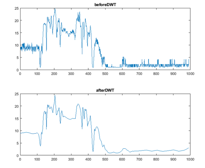
yd=wden(subcarrier,'heursure','s','one',10,'sym3');

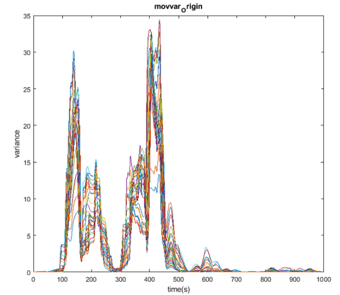
vs=movvar(yd,50)

figure(1)
subplot(2,1,1);
plot(subcarrier);
title('beforeDWT');
subplot(2,1,2);
plot(yd);
title('afterDWT');
figure(9)
plot(vs);
xlabel('time(s)');
ylabel('variance');
title('movvar_Origin');
hold on

Hall(:,j)=yd.';
end

%uncentralize
for k=1:30
    for i=1:990
    Zk(i)=Hall(i,k)-mean(Hall(:,k));
    end
    Z(:,k)=Zk;
end

%Z covariance
C=cov(Z);
% Eigenvector e, eigenvalue R
[E,R]=eig(C);
R=ones(1,30)*R;%The eigenvalues generated by the eig function are transformed into row vectors

TZ_ER=[R;E];
TZ_ER=TZ_ER';
%The eigenvectors are arranged in descending order according to the size of R
TZ_ER=sortrows(TZ_ER,1,'descend');
R=TZ_ER(:,1);%Separating eigenvalues
E=TZ_ER(:,2:end);%Separating eigenvectors
Pca=zeros(30,1);
E=E'
Pca=E(:,1);%chose the 1st pinciple component
Y=Hall*Pca;

 res=sum(R(1:2))/sum(R);

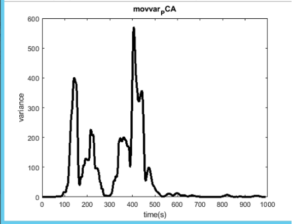
apv=movvar(Y',50)
figure(2)
plot(apv,'k','linewidth',3);
xlabel('time(s)');
ylabel('variance');
title('movvar_PCA');
figure(15)
plot (Y,'linewidth',3);
hold on
title('afterPCA');

 fprintf('consists the percent\n',res*100);
for i=1:30
plot(Hall(:,i));
end

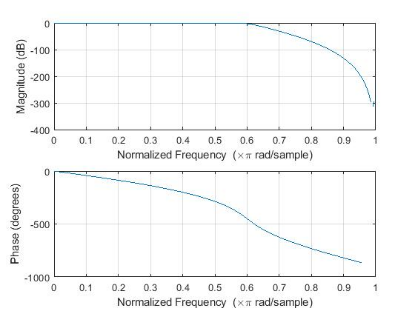
Butterworth
hfc = 300; 
lfc = 0;
fs = 1000;
order = 10;

[b,a] = butter(order, hfc/(fs/2));
figure(5)
freqz(b,a)
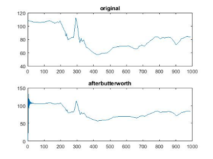
noisy_sig = D{7};
dataIn = randn(1000,1);
dataOut = filter(b,a,Y);
figure(6)
subplot(2,1,1)
plot(Y)
hold on
title('original');
subplot(2,1,2)
plot(dataOut);
hold on
title('afterbutterworth');
Y=dataOut;

FFT
F=fft(Y,1024);
figure(9)
plot(abs(F));
axis([0 1800 0 1500]);
STFT
fs = 1000;%
window = 512;
noverlap = window/2;
nfft=1024;

f_len = window/2 + 1;
f = linspace(0, 150e3, f_len);
% s= spectrogram(Y, window, noverlap);
% figure(1);
% imagesc(20*log10((abs(s))));xlabel('Samples'); ylabel('Freqency');
% colorbar;

[s, f, t, p] = spectrogram(Y, window, nfft, f, fs);
figure(8);
imagesc(t, f, p);xlabel('Samples'); ylabel('Freqency');
colorbar;

[s, f, t] = spectrogram(Y, 512,256,f, fs);
figure;
imagesc(t, f, 20*log10((abs(s))));xlabel('Samples'); ylabel('Freqency');
colorbar;

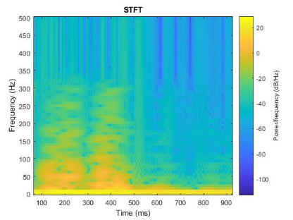
figure(16)
subplot(2,1,1)
 spectrogram(Y,128,127,128,fs,'yaxis'); 
  title('STFT');
 hold on
[s,f,t,ps]=spectrogram(Y,64,63,64,fs,'yaxis');
 m=4:33
 n=1:927
 pmax=max(ps(m,n),[],1);
 subplot(2,1,2)
% % figure(17)
 plot(pmax,'linewidth',3,'MarkerEdgeColor','k','MarkerFaceColor','g','MarkerSize',10);
 hold on
 title('power curve');
1
2
3
4
5
6
7
8
9
10
11
12
13
14
15
16
17
18
19
20
21
22
23
24
25
26
27
28
29
30
31
32
33
34
35
36
37
38
39
40
41
42
43
44
45
46
47
48
49
50
51
52
53
54
55
56
57
58
59
60
61
62
63
64
65
66
67
68
69
70
71
72
73
74
75
76
77
78
79
80
81
82
83
84
85
86
87
88
89
90
91
92
93
94
95
96
97
98
99
100
101
102
103
104
105
106
107
108
109
110
111
112
113
114
115
116
117
118
119
120
121
122
123
124
125
126
127
128
129
130
131
132
133
134
135
136
137
138
139
140
141
142
143
144
145
146
147
148
149
150
151
152
153
154
155
156
157
<
登录后即可复制

整段代码效果如下图：